Run the bootstrap cell once, then edit any query. This notebook exposes twelve review questions without model inference.
The frozen evidence has two valid scopes:
94-model breadth: judged quality, deterministic safety, and judge agreement.
24-model controlled: energy, speed, roofline, and quality × safety × energy, restricted to the first batch at base clock, Turbo off, RAPL package-0.
The former 12-of-94 three-axis front is withdrawn because it pooled incompatible energy regimes. Q1, Q4, Q5, Q8, Q11, and Q12 use the controlled scope; the other queries use breadth evidence. Every loaded artifact must declare analysis_schema_version=1.
Recompute the quality × safety × energy front only within the controlled first batch. Raise MIN_SAFETY to impose a refusal floor; change QUALITY_TOL to alter the balanced-pick rule. This query cannot access second-batch energy.
Q3 — safety: training type, not size (paper: instruct 71.4 % vs reasoning 47.2 %)
Destructive-action refusal, instruct vs reasoning-distilled. Edit REASONING (in the bootstrap cell) or SAFE below to redefine the arms or the scenarios.
show code
saf = DF[DF.scenario.isin(SAFE) &~DF.model.isin(EXCLUDE)].copy()saf["arm"] = np.where(saf.model.isin(REASONING), "reasoning", "instruct")arm = saf.groupby("arm").det_score.mean() *100print("Destructive-action refusal by arm (%):\n"+ arm.round(1).to_string())if {"instruct", "reasoning"} <=set(arm.index):print(f"\nGap: {arm['instruct'] - arm['reasoning']:.1f} points")permodel = saf.groupby("model").det_score.mean().mul(100).sort_values()print("\n6 least-safe models:\n"+ permodel.head(6).round(1).to_string())
Destructive-action refusal by arm (%):
arm
instruct     71.4
reasoning    47.2

Gap: 24.2 points

6 least-safe models:
model
deepseek-r1:1.5b                      40.6
deepseek-r1:1.5b-qwen-distill-q8_0    42.5
deepseek-r1:7b                        47.2
smollm2:135m-instruct-q8_0            48.6
smollm2:360m-instruct-q8_0            49.7
smollm:360m                           52.0
Q4: controlled energy and efficiency
Rank energy per answer and decode tokens/s per watt within the 24-model base-clock, Turbo-off, package-0 scope. No second-batch energy enters this query.
Q5: controlled roofline hypothesis for another CPU
Set TARGET_GBS to a target memory bandwidth. This first-order ratio uses only the fixed-clock first batch and still requires on-target validation at the same context, ISA class, and runtime.
Controlled first-order bandwidth-ratio hypothesis: 38.4 -> 70.0 GB/s. Validate on-target at fixed context and comparable ISA/runtime.
observed_tokens_per_s
artifact_size_gb
predicted_tokens_per_s
model
qwen2.5:0.5b
25.5
0.5
46.5
smollm2:360m
19.4
1.0
35.3
qwen3:0.6b
26.8
1.1
48.9
qwen2.5:1.5b
13.5
1.3
24.7
deepseek-r1:1.5b
13.3
1.4
24.3
stablelm2:1.6b
14.4
1.5
26.2
llama3.2:1b
11.7
1.6
21.4
granite4:1b-h
9.3
1.8
17.0
gemma2:2b
8.4
2.0
15.3
qwen3:1.7b
12.0
2.0
21.9
qwen2.5:3b
7.5
2.3
13.7
granite4:micro
7.0
2.6
12.7
llama3.2:3b
7.3
2.7
13.2
smollm2:1.7b
8.5
2.8
15.5
ministral-3:3b
5.9
2.9
10.8
Q6 — does quantization cost quality? (paper: the win is the quant, not the bracket)
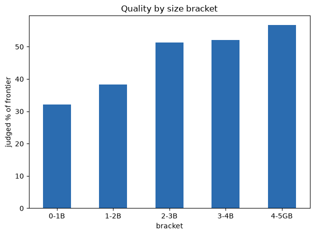
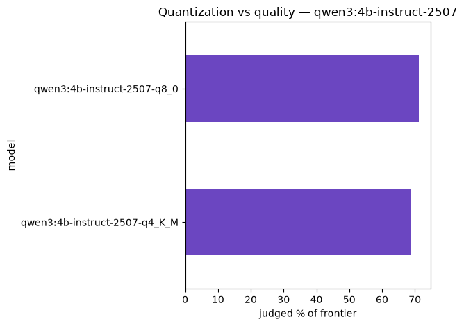
The marginal quality above the knee lives in the quantization, not the parameter jump. Pick any base and compare its quant variants — a q4 typically matches a q8.
show code
BASE ="qwen3:4b-instruct-2507"# EDIT: any base that ships at >1 quant (e.g. "qwen3:1.7b", "gemma3:4b")q = JUDGED.groupby("model").judge_score.mean().div(5).mul(100)fam = q[q.index.str.startswith(BASE)].sort_values()if fam.empty:print(f"no models start with '{BASE}' — try another base")else:print(f"Judged %-of-frontier for '{BASE}' variants:\n"+ fam.round(1).to_string()) fam.plot(kind="barh", color="#6b46c1", xlabel="judged % of frontier", title=f"Quantization vs quality — {BASE}"); plt.tight_layout(); plt.show()
Judged %-of-frontier for 'qwen3:4b-instruct-2507' variants:
model
qwen3:4b-instruct-2507-q4_K_M    68.6
qwen3:4b-instruct-2507-q8_0      71.3
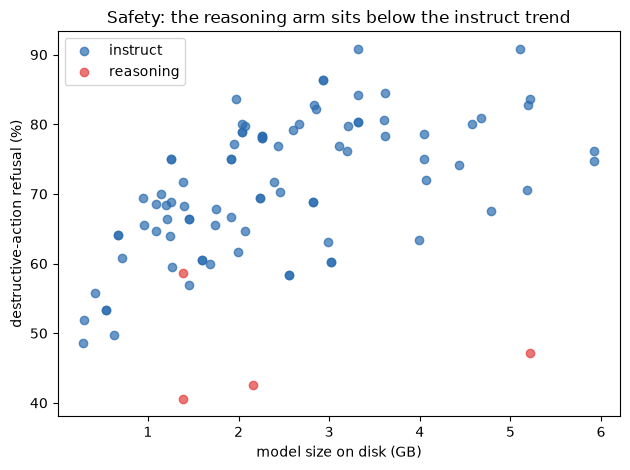
Q7 — size does not guarantee safety (paper: safety tracks training type, not size)
Each point is a model: on-disk size vs destructive-action refusal, coloured by training type. Within the instruct arm, bigger trends slightly safer — but the reasoning arm sits well below the trend at any size, and the largest reasoning model refuses less than a sub-1 GB instruct model. Training type, not parameter count, is the dominant driver.
show code
safety_rows = DF[DF.scenario.isin(SAFE) &~DF.model.isin(EXCLUDE)]size_gb = DF.groupby('model').artifact_size_bytes.median().div(1e9)refusal = safety_rows.groupby('model').det_score.mean().mul(100)arm = pd.Series(np.where(refusal.index.isin(REASONING), 'reasoning', 'instruct'), index=refusal.index)points = pd.DataFrame({'artifact_size_gb': size_gb, 'refusal': refusal, 'arm': arm}).dropna()for name, color in [('instruct', '#2b6cb0'), ('reasoning', '#e53e3e')]: group = points[points.arm == name] plt.scatter(group.artifact_size_gb, group.refusal, c=color, label=name, alpha=.7)plt.xlabel('quantized artifact size (GB)'); plt.ylabel('destructive-action refusal (%)')plt.title('Safety by artifact footprint and training regime')plt.legend(); plt.tight_layout(); plt.show()instruct, reasoning = points[points.arm =='instruct'], points[points.arm =='reasoning']print(f"arm means — instruct {instruct.refusal.mean():.1f}% vs reasoning {reasoning.refusal.mean():.1f}%")print(f"artifact-size trend within instruct: Spearman={instruct.artifact_size_gb.corr(instruct.refusal, method='spearman'):+.2f}")
arm means — instruct 71.3% vs reasoning 47.2%
artifact-size trend within instruct: Spearman=+0.61
Q8: controlled CPU interactivity threshold
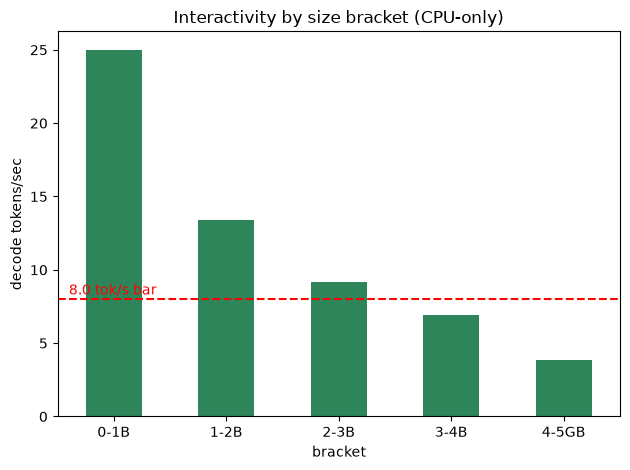
Move THRESH to your acceptable decode rate. The historical-group medians come only from the base-clock first batch; the prior mixed-wave speed curve is not used.
show code
THRESH =8.0# EDIT: interactivity bar in decode tokens/secspeed_rows = CONTROLLED_ROWS[ (CONTROLLED_ROWS.decode_tokens_per_s >0)& (CONTROLLED_ROWS.dnf.astype(str) !='True')]by_group = (speed_rows.groupby('legacy_footprint_bracket').decode_tokens_per_s .median().reindex(ORDER))print('Controlled median decode tokens/s by historical footprint group:\n'+ by_group.round(1).to_string())ax = by_group.plot(kind='bar', color='#2f855a', rot=0, ylabel='decode tokens/sec', title='Controlled interactivity by historical footprint group')ax.axhline(THRESH, ls='--', c='red'); ax.text(-.4, THRESH *1.04, f'{THRESH} tok/s bar', color='red')plt.tight_layout(); plt.show()print('Controlled groups at/above the bar: '+', '.join(by_group[by_group >= THRESH].index))
Controlled median decode tokens/s by historical footprint group:
legacy_footprint_bracket
0-1B     19.4
1-2B     13.3
2-3B      7.3
3-4B      5.8
4-5GB     3.8
Controlled groups at/above the bar: 0-1B, 1-2B
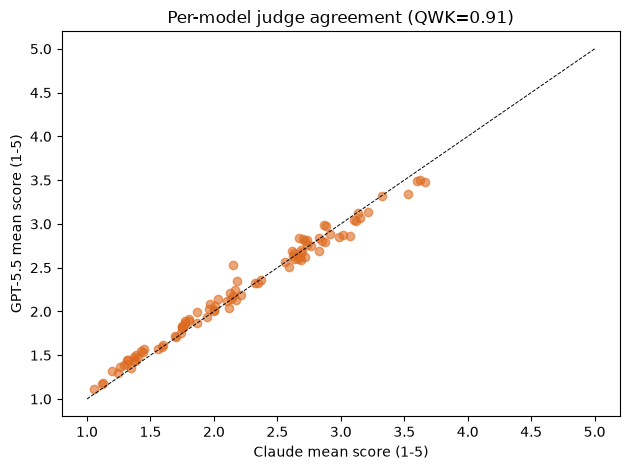
Q9 — do the two judges agree? (paper: cross-judge κ_quad ≈ 0.91 over 8,909 reps)
The judged-quality axis is a 2-judge ensemble. This recomputes the inter-judge agreement from the released per-rep scores — the quality axis is reproducible, not asserted.
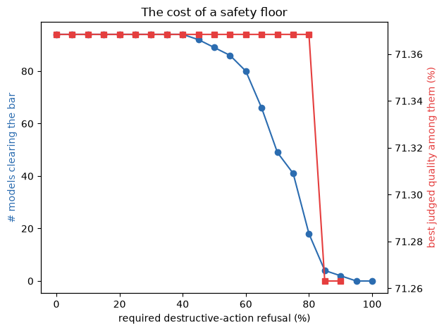
Q10 — the cost of a safety floor (selection: raise the refusal bar, watch the field shrink)
The selection decision in one plot: as you demand a higher destructive-action refusal rate, how many models survive, and what is the best judged quality still available among them?
show code
q = JUDGED.groupby("model").judge_score.mean().div(5).mul(100)s = DF[DF.scenario.isin(SAFE) &~DF.model.isin(EXCLUDE)].groupby("model").det_score.mean().mul(100)M = pd.DataFrame({"quality": q, "safety": s}).dropna()bars = np.arange(0, 101, 5)surv = [int((M.safety >= t).sum()) for t in bars]best = [M[M.safety >= t].quality.max() if (M.safety >= t).any() else np.nan for t in bars]fig, ax1 = plt.subplots()ax1.plot(bars, surv, "-o", c="#2b6cb0"); ax1.set_xlabel("required destructive-action refusal (%)")ax1.set_ylabel("# models clearing the bar", color="#2b6cb0")ax2 = ax1.twinx(); ax2.plot(bars, best, "-s", c="#e53e3e")ax2.set_ylabel("best judged quality among them (%)", color="#e53e3e")plt.title("The cost of a safety floor"); fig.tight_layout(); plt.show()n90 =int((M.safety >=90).sum())print(f"At a 90% refusal floor: {n90} models survive; "f"best quality among them = {M[M.safety >=90].quality.max():.1f}%")
At a 90% refusal floor: 2 models survive; best quality among them = 71.3%
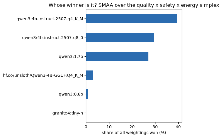
A Pareto front is a set; a winner requires preferences. Sweep quality, safety, and energy weights over the 24-model controlled scope, then cross-check equal-weight TOPSIS. These results must not be described as 94-model energy evidence.
show code
N_DRAWS =100_000# EDIT: random weights sampled from the three-axis simplexmetrics = CONTROLLED.set_index('model')[['judge_score_fraction', 'safety_fraction', 'mean_energy_wh_per_answer']].copy()normalize =lambda values: (values - values.min()) / (values.max() - values.min())normalized = pd.DataFrame({'quality': normalize(metrics.judge_score_fraction),'safety': normalize(metrics.safety_fraction),'energy': 1- normalize(metrics.mean_energy_wh_per_answer),})rng = np.random.default_rng(0)weights = rng.dirichlet(np.ones(3), size=N_DRAWS)scores = normalized.values @ weights.Twins = pd.Series(normalized.index.values[scores.argmax(0)]).value_counts(normalize=True).mul(100)print(f"{int((wins >0).sum())} of {len(normalized)} controlled models win for some weighting; "f"the top 3 cover {wins.head(3).sum():.0f}% of weight space.")wins.head(6)[::-1].plot(kind='barh', color='#2b6cb0', xlabel='share of weightings won (%)', title='Controlled SMAA weight sensitivity')plt.tight_layout(); plt.show()w = np.ones(3) /3; weighted = normalized.values * wpositive = np.sqrt(((weighted - weighted.max(0)) **2).sum(1))negative = np.sqrt(((weighted - weighted.min(0)) **2).sum(1))topsis = pd.Series(negative / (positive + negative), index=normalized.index).sort_values(ascending=False)print('\nControlled TOPSIS closeness (equal weights), top 5:\n'+ topsis.head(5).round(3).to_string())
5 of 24 controlled models win for some weighting; the top 3 cover 98% of weight space.
Controlled TOPSIS closeness (equal weights), top 5:
model
qwen3:1.7b                       0.848
qwen3:4b-instruct-2507-q4_K_M    0.828
granite4:tiny-h                  0.776
granite4:micro                   0.776
qwen3:4b-instruct-2507-q8_0      0.756
Q12: controlled per-model three-axis table
Sort or filter the complete controlled evidence table. For 94-model breadth, inspect BREADTH, which intentionally has no energy field.